core module
These functions allows to open/read three type of data: native febus file, reducted file or ZMQ socket data stream. Data can be read with different parameters that allow to define time/space range, time/space decimation, etc
The module relies upon two classes:
A1File to deal with files
A1Section to deal with data once a file has been read
Basic functions/methods
- core.open(filename, format=None, verbose=1)
Description
Open a Febus das file, a reducted Hdf5 file or a socket stream on a DAS-A1 Febus interrogator and return an A1File instance
Input/Return
- filename:
(str) a filename or a socket address in the form “tcp://ip_address:port”
- format:
(str) one of ‘febus’, ‘reducted’, ‘socket’. If not supplied, the function tries to determine it automatically
The socket address can be formatted using the a1das.tcp_address utility
- return:
a A1File class instance
Usage example
>>> import a1das
>>> f = a1das.open('my_filename', format='reducted')
>>> f2 = a1das.open(a1das.tcp_address('128.0.0.1',6667), format='socket')
- A1File.read(block=None, trange=None, drange=None, verbose=0, float_type='float64', tdecim=1, ddecim=1, **kwargs)
Description
Read data from a Febus/reducted file or a socket directly connected to Febus DAS in memory and return a A1Section class instance.
All data are read unless one of the three options is set: block, trange, drange. block is exclusive with trange,drange and return data aligned on block limits
Data are read as float32 and are converted by default as float64 unless specified
Input/Return for all file format
- trange:
(list/tuple) time range to be read, see
parse_trange()for format (default = None, read all)- drange:
(list/tuple) distance range to be read, see
parse_drange()for format (default = None, read all)- verbose:
(int) verbosity level
- float_type:
‘float_32’ or ‘float_64’ float type for data in memory, default is float64
- Return:
A A1Section class instance
Input febus file
- block:
(list), block=[start, end, step]. Read full block of data, from start to end by step. [0,0,?] read all blocks [] read one block default = None
- ddecim:
(int) decimation along spatial dimension, (default 1, must be a divider of chunck/block size)
Input reducted file and transposed data
- tdecim:
(int) time decimation (default 1)
Usage example
>>> import a1das
>>> f = a1das.open("my_filename", format='febus')
>>> a1 = f.read(trange=(0.,1800.),drange=(100., 900.),skip=False) #select by time and distance
>>> a2 = f.read(trange=range[0,100]) #select by indices
More functions and classes
A1File class
This class is used to initiate I/O operations on files and it allows to inspect all metadata without reading all content
- class core.A1File(file_header=None, socket_header=None, data_header=None)
Description
A1File class contains file/socket descriptors to read and convert DAS data from Febus format, or H5 reducted file format or data socket stream (ZMQ protocol).
Class content
A1File.file_header: file header (_A1FileHeader class instance)
A1File.socket_header: socket header (_A1SocketHeader class instance)
A1File.data_header: metadata (dict)
The metadata list is obtained by typing the name of the A1File instance (see example below)
Reading/setting data_header metadata
Read directly as a dictionnary from A1File instance (ex: f[‘dt’]) or from data_header member (ex: f.data_header[‘dt’])
Set by the
set_item()method ex: f.set_item(dt=0.1) or through data_header ex: f.data_header[‘dt’]=0.1Usage example
>>> import a1das
>>> f = a1das.open("my_filename")
>>> f # print metadata header values
>>> GL = f['gauge_length']
>>> f.set_item(gauge_length=10.)
A1Section class
This class is the container to manipulate metadata and data with a number of utility functions/methods
- class core.A1Section(header=None, data=None)
Description
A1Section class contains das data and metadata read from file or TCP stream.
Class content
- A1Section.data:
2D float array (ndarray of shape [ntime x nspace] or [nspace x ntime]) or
4 x 2D int8 array (ndarray of shape |4 x ntime x nspace]) for febus RAW data
- A1Section.header:
dictionary that contains metadata.
metadata (header), Reading/setting
The metadata content is initialized using the _A1DataHeader class to control the content and impose a minimum set of metadata
Minimum header content that is “defined” as mandatory can by viewed using
min_header()Read directly as a dictionnary from A1Section ex: a1[‘dt’] or through data_header ex: a1.header[‘dt’]
Set by the
set_item()method, ex: a1.set_item(dt=0.1) or through data_header ex: a1.header[‘dt’]=0.1See example below
Usage example
>>> import a1das
>>> f=a1das.open(filename)   # open file
>>> a1 = f.read()            # read section
>>> a1                       # print header values in a nice fashion
>>> a1.header                # return header as a dictionary
>>> time_step=a1['dt']       # get time step
>>> a1.set_item(dt=0.1)      # set time step
>>> a1.header['dt']=0.1      # same as above
>>> array = a1.data          # copy data array in numpy array
>>> time = a1['time']        # copy the time vector in a numpy array
>>> dist = a1['dist']        # copy the distance vector in a numpy array
Plotting A1Section
- A1Section.plot(fig=None, clip=100, splot=(1, 1, 1), title='', max=100, amax=None, by_trace=False, variable_area=False, drange=None, trange=None, redraw=None, **kwargs)
Description
Produce a vector plot of the das section, optionnaly with variable area
Input/Return
- fig:
figure handle (default None)
- clip:
(int) clip amplitude at clip% of the max amplitude (default 100%)
- splot:
(tupple) plot as a subplot (default subplot(1,1,1))
- title:
(str) figure title (default None)
- max:
(int) maximum number of traces on the plot (default 100)
- amax:
maximum amplitude for clipping if not using clip percentage (default None)
- by_trace:
(bool) normalize by plot (False) or by trace (True) (default = False)
- variable_area:
(bool) plot with variable_are (half wiggle is filled in black) (default False)
- drange:
(tupple) distance range [dmin, dmax]
- trange:
(tupple) time range [tmin, tmax]
- redraw:
{lines} redraw lines of a precedent figure or None for new plot, requires fig argument
- rtype:
figure_handle, curve_list
Usage example
>>> import a1das
>>> f=a1das.open(filename)
>>> a1=f.read()
>>> a1.plot(clip=50,variable_area=True)
- A1Section.rplot(fig=None, cmap='RdBu', vrange=None, splot=(1, 1, 1), title='', drange=None, trange=None)
Description
Produce a raster plot of the das section
Input
- fig:
figure handle (default None)
- cmap::
colormap (default=RdBu)
- vrange:
trace amplitude range (default None)
- splot:
plot as a subplot (default subplot(1,1,1))
- title:
figure title (default None)
- drange:
distance range
- trange:
time range
- rtype:
figure_handle, axes_handle
Usage example
>>> import a1das
>>> f=a1das.open(filename)
>>> a1=f.read()
>>> a1.rplot()
A1Section to obspy_stream or xarray
and more A1Section methods
- A1Section.save(filename, **kwargs)
Description
a.save(filename)
Save a A1Section in a file using the reducted file format.
Input
- filename:
a name for the hdf5 file that contains the reducted file
Usage example
>>> import a1das
>>> f = a1das.open('my_filename', format='febus')
>>> a = f.read(trange=(tmin,tmax), drange=(dmin,dmax), skip=False) # read and extract a subportion of the original file
>>> a.save('new_section') # 'a' can be read later using the same a1das.open() and f.read() functions
>>> f.close()
- A1Section.synchronize()
Description
This function is similar to the synchronize command in SAC. Set the origin time (field ‘otime’ in data header) to the time of the first sample in the section. After this operation, the value of time[0] is equal to 0.
- A1Section.is_transposed()
Description
Only relevant for <reducted> format, return True if the data are transposed in file from the original Febus format. Transposed = the data array is stored as data[nspace, ntime], Not transposed = the data array is stored as data[ntime, nspace],
- returns:
False for Febus original files, True/False for reducted files
- A1Section.concat(b)
Description
a.concat(b): Concatenate section b behind section a along the fast axis if a and b are ordered as [space x time], fast axis is time and on obtain a new section [ space x 2*time] if a and b are ordered as [time x space], not implemented
- returns:
a new section
- A1Section.index(drange=None, trange=None)
Description
Return the index or list of indices that correspond(s) to the list of distance(resp. time) range in the ‘distance’ vector (resp. time vector)
Input
Only one of trange or drange can be given
- drange:
(list or tuple) see
parse_drange()for format- trange:
(list or tuple) see
parse_trange()for format- returns:
A list of indices that match the given range in the A1Section.data_header[‘dist’] or
A1Section.data_header[‘time’] vectors
Usage example
————-
>>> import a1das
>>> f=open(‘filename’)
>>> a=f.read()
>>> dlist1 = a.index(drange=50.) # get index for distance 50.m
>>> dlist1 = a.index(drange=[50.]) # get index at distance 50 m
>>> dlist2 = a.index(drange=[50., 60.]) # get 2 indices at 50 and 60m
>>> dlist3 = a.index(drange=[[dist] for dist in np.arange(50,60.,1.)]) # get all indices for distance 50< ..<60 every 1m
>>> dlist4 = a.index(drange=(50.,60.)) # get all indices between 50. and 60.m
>>> tlist = a.index(trange=[10., 20.]) # 2 indices for time 10s and 20 sec after 1st sample
>>> tlist = a.index(trange=[2020 (03:12-10:10:10, 2020:03:12-10:10:20]))
- A1Section.set_item(**kwargs)
Description
Update/create a header entry in the data_header class dictionnary attached to A1Section
Input
- kwargs:
arbitrary list of key_word = value
Usage example
>>> import a1das
>>> f=a1das.open(filename)
>>> a=f.read()
>>> a.set_item(cat_name='medor',cat_food='candies',cat_age=7)
- classmethod A1Section.min_header()
Description
Display the mandatory header fields of the A1Section class metadata. There can be additional fields inserted using
set_item()but the following fields must be filled when creating an instance of A1Section as well as when writing a reducted file.The list of mandatory fields is defined in _a1headers.py by the “_required_header_keys” dictionary
Internals
- core.parse_trange(dhd, trange)
Description
Convert various input time range formats into a unified form for internal use
Input
- dhd:
header from A1File.data_header or A1Section.header
- trange::
(list, tuple or range) acceptable time range formats are:
[start, end]/[single_value]: where value(s) are sec from 1st sample:
range(istart, iend): where values are time array index
[date1, date2]: where date? is a string=’YYYY:MM:DD-hh:mn:ss’, or an obspy.UTCDateTime object
None: read all
!!!! if specifying a single time, use list as [start] or tuple as (start,)
- returns:
trange = [start, end]
- rtype:
list with time range relative to first sample
- core.parse_drange(dhd, drange)
Description
Convert various input distance range formats into a unified form for internal use
Input
- dhd:
data_header from A1File.data_header or A1Section.header
- drange:
(list, tuple or range) acceptable time range formats are:
[start, end]/[single_value]: where value(s) are meters from space origin:
range(istart, iend): where values are time array index
None: read all
!!!! if specifying a single distance, use list as [start] or tuple as (start,)
- returns:
drange = [start, end]
- rtype:
list with time range starting/ending distance with respect to first location
- core.tcp_address(address='127.0.0.1', port=6667)
Return a string of the form <tcp://address:port> from an IP address and a port number Input —–
- Address:
IP adress as a string, default to ‘127.0.0.1’
- Port:
IP port default to 6667
About Febus-Optics DAS-A1 file format
This format uses HDF5 container and defines several groups; datasets; group attributes; dataset attributes. This paragraph documents the Version 2.3.5 of the format.
H5 organization
Abbreviations: G=group only, GA=Group with attributes, D=Dataset only, DA=Dataset with attributes
                    localhost.localdomain(G)
                             |
                             |
                             ---         .....             -----         ....
                             |                               |
                             |                               |
                          Source1(GA)                     SourceK
                             |
                             |
                   --------------------     ....       -----
                   |                  |                  |
                   |                  |                  |
                 time(D)           Zone1(GA)          ZoneK
                                      |
                                      |
                              -----------------------------    .....
                              |                |
                              |                |
                           Channel1(D)      Channel2(D)
Metadata are stored as group attributes. There are Source attributes and Zone attributes which respectively contains the following informations (some data are duplicated, e.g. Version):
Source Attributes:
‘AmpliPower’, ‘BlockOverlap’, ‘BlockRate’, ‘DataDomain’, ‘FiberLength’, ‘Hostname’, ‘Oversampling’, ‘PipelineTracker’, ‘PulseRateFreq’, ‘PulseWidth’, ‘SamplingRate’, ‘SamplingRes’, ‘Version’, ‘WholeExtent’
# Example for reading Source attribute using h5py:
>>> import h5py
>>> f = h5py.File('my_file.h5')
>>> blockRate = f['localhost.localdomain/Source1'].attrs['BlockRate']
Zone attributes:
‘AmpliPower’, ‘BlockOverlap’, ‘BlockRate’, ‘Components’, ‘DataDomain’, ‘DerivationTime’, ‘Extent’, ‘FiberLength’, ‘GaugeLength’, ‘Hostname’, ‘Origin’, ‘Oversampling’, ‘PipelineTracker’, ‘PulseRateFreq’, ‘PulseWidth’, ‘SamplingRate’, ‘SamplingRes’, ‘Spacing’, ‘Version’
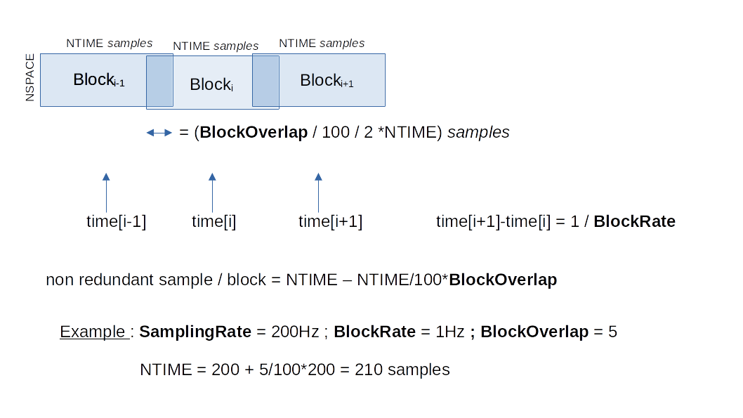
Data are stored in datasets localhost.localdomain/Source?/Zone?/Channel?. There are as many datasets as channels acquired simultaneously. Each dataset contains an array of dimension [NBLOCK x NTIME x NSPACE]. Each block contains NTIME time samples and NSPACE channel samples. Blocks are written at the <BlockRate> frequency, and they overlap with a <BlockOverlap> percentage.
Time information is stored in dataset localhost.localdomain/Source?/time. This vector contains the absolute time for each of the NBLOCK block of data.
# Example for reading time vector using h5py:
>>> import h5py
>>> f = h5py.File('my_file.h5')
>>> block_times = f['localhost.localdomain/Source1/time'][:]
Time block storage scheme: the following diagram displays how data is written by block.